Paper: Seismic Roots
Using \(V_p\) and \(V_s\) to Characterize the Spatial Extent of Shear Strengthening Under a Longleaf Pine
Key Points
P-wave (\(V_p\)) and S-wave (\(V_s\)) velocities can be used to study the rooting zone under trees.
Soil modified by roots caused an increase in shear strength under the tree, resulting in low \(V_p\)/\(V_s\) values.
Low \(V_p\)/\(V_s\) values indicate tree-modified soil in the region where normal shear failure from vertical loading is likely to occur.
Introduction
Trees are the tallest freestanding structures in nature and populate nearly every landscape on Earth. Some trees reach heights exceeding 120 m (Tredici 1999; Hickey, Kostoglou, and Sargison 2000), while others stand for thousands of years (Currey 1965). Trees are slender, top-heavy, and inherently unstable (Sellier and Suzuki 2020). Due to their towering heights and expansive canopies, it is often assumed that tree roots mirror the canopy structure and extend deep into the soil. However, a global compilation of tree rooting depths indicate that this assumption is generally incorrect (Canadell et al. 1996; Jackson et al. 1996). Although roots have been reported at depths of up to 68 m, the average rooting depth is only 7.1 \(\pm\) 1.2 m (n = 82) (Canadell et al. 1996). Furthermore, global observations show that 86% of a tree’s roots are located within the top 30 cm of soil (Jackson et al. 1996).
Despite their shallow depth, roots anchor trees to the soil, enabling them to grow upright against gravity and resist lateral wind loads (Sellier and Suzuki 2020; Ancelin, Courbaud, and Fourcaud 2004; Dupuy et al. 2007). Roots often distribute themselves asymmetrically around the tree to compensate for additional lateral loading caused by slopes (Taufiqurrachman et al. 2023) and to counteract forces from prevailing winds (Montagnoli et al. 2019). Individual roots also adapt structurally as they grow, forming I-beams or T-beams to enhance mechanical support (Danjon, Fourcaud, and Bert 2005; Dumroese et al. 2019). As roots develop, they modify the soil’s mechanical properties by increasing its shear strength (Giadrossich et al. 2017). Shear strength is defined as the maximum shear stress the soil can withstand before failure.
The Mohr-Coulomb failure criterion is one of the simplest and most widely used models for describing soil failure (Labuz and Zang 2012). It defines shear strength using two quantifiable properties: (1) soil cohesion (\(C\)) and (2) the internal angle of friction (\(\phi\)). Materials with higher cohesion and friction angles exhibit greater shear strength. Direct shear tests on soils with and without roots have shown that rooted soils possess higher shear strength than unrooted soils (Giadrossich et al. 2017). This increase is attributed to the tensile strength of roots, which act as reinforcing elements and enhance soil cohesion. As a result, soil–root systems exhibit increased strength, even under zero confining stress (Abe and Ziemer 1991; Li et al. 2024; Jian et al. 2024). Increases in cohesion have been observed when roots were embedded in a soil matrix (Tomobe et al. 2023; Ghestem et al. 2014; Stokes et al. 2009), collected from field samples (Li et al. 2024; Jian et al. 2024), and grown in shear boxes for up to ten months (Ali and Osman 2008).
The magnitude of shear strength enhancement depends on the root area and diameter and the orientation relative to the shear failure plane (Ghestem et al. 2014). Existing methods for measuring shear strength are typically conducted on small volumes, often just a few cubic centimeters. To increase sample volume, plants have been grown in large testing apparatuses measuring several hundred cubic centimeters (Ali and Osman 2008). Additionally, root pullout and overturning tests, performed both in situ and in laboratory settings, have investigated tree failure mechanisms (Kevern and Hallauer 1983; Docker and Hubble 2008; Mickovski and Ennos 2002). However, the destructive nature of these tests, combined with unknown root architecture and uncertain biomechanical properties, leaves many questions unanswered about how external loads are transferred through roots into the soil. Currently, a non-destructive method does not exist to characterize the mechanical impact of roots in situ under living trees.
This lack of methodology exists because roots are difficult to characterize without harming the tree (Miller, Allen, and Maier 2006). Non-invasive technologies for root characterization include sonic root tools (Proto et al. 2020) and electrical resistivity methods (Robinson, Slater, and Schäfer 2012; Ehosioke et al. 2020). Among these, ground-penetrating radar (GPR) offers the highest resolution and can produce detailed maps of coarse roots to depths of a few centimeters (Hruska, Čermák, and Šustek 1999; Butnor et al. 2001; Guo et al. 2013; Zajícová and Chuman 2019). However, GPR is limited to detecting shallow lateral roots and cannot resolve roots located directly beneath the trunk. Vertical roots directly below the tree are particularly difficult to characterize because they are obscured by both soil and the tree trunk, yet they are critical for tree stability. For example, the taproot of marine pine trees in France accounts for over 60% of strain under large lateral loads (M. Yang et al. 2014). Additionally, extracted 3D root networks of pines reveal multiple vertically oriented roots forming a cage-like structure around the taproot, which enhances soil shear strength (Danjon, Fourcaud, and Bert 2005; Brantley et al. 2011; M. Yang et al. 2014; X.-D. Yang et al. 2019; Dumroese et al. 2019). Despite its resolution, GPR cannot quantify the mechanical effects of roots on soil, and vertical roots beneath the trunk remain unmeasured.
Seismic refraction is a promising non-invasive, near-surface geophysical method. It can characterize the soil-root composite directly beneath the trunk without harming the tree. Over the past decade, seismic refraction, particularly travel-time tomography, has proven to be a powerful tool. It has imaged subsurface structures beneath hillslopes (Zelt et al. 2013; Sheehan, Doll, and Mandell 2005; Befus et al. 2011; Holbrook et al. 2014) and watersheds (Brady A. Flinchum et al. 2018; Uecker et al. 2023). In isotropic elastic materials, seismic velocities are governed by compressibility, shear resistance, and density. Thus, velocities depend on the mechanical properties of the soil-root matrix at small strains.
This study aimed to investigate the relationship between root structure and soil shear strength using high-resolution seismic refraction surveys. At the South Carolina Botanical Gardens, two profiles of P-wave (\(V_{p}\)) and horizontally polarized S-wave (\(V_{s}\)) velocities were collected around a 31 m tall longleaf pine (Pinus palustris). The results showed minimal changes in \(V_{p}\), but increases in \(V_{s}\) produced low (\(V_{p}/V_{s}\)) values (<1.5) directly beneath the tree. The increased \(V_{s}\), suggested that vertical roots beneath the trunk increased the soil’s shear stiffness. The minimal changes in \(V_{p}\) indicated that the soil was not compressed and likely remained porous. Additionally, the structure of the (\(V_{p}/V_{s}\)) values resembled the expected shear failure envelope defined by the Prandtl Wedge (Van Baars 2018). This similarity supports the hypothesis that the tree may opportunistically grow roots to reinforce soil along the shear failure plane, enabling continued growth.
Methods
Three methods were used in this study. Structure-from-Motion (SfM) was employed to generate a localized, high-resolution digital elevation model (DEM) and a 3D point cloud. Two perpendicular shallow seismic refraction profiles were collected, with the largest tree in the study positioned at their intersection. \(V_{p}\) and \(V_{s}\) velocities were calculated using travel-time tomography by inverting the first arrivals of P-waves and transversely polarized S-waves (Figure 1). Finally, the resulting \(V_{p}\) and \(V_{s}\) values were compared to the structures predicted by the general shear failure envelope defined by Prandtl’s Wedge (Van Baars 2018).
Structure from Motion
SfM was used to construct a high-resolution DEM with a spatial resolution of 2 cm. The SfM model was generated from 425 photographs taken with a Mavic Air 2 drone. Approximately 65% (275 of 425) of the photos were captured at low elevation, with the camera oriented directly toward the ground. The remaining 150 photographs were used to estimate the aboveground structure. Agisoft Metashape, a semi-automatic photogrammetry software, inverted for camera positions and orientations by identifying common features in overlapping images (Metashape?; Lowe 1999). Once the position and orientation of each photo were known, pixels from each image were reprojected into 3D space (Westoby et al. 2012; Micheletti, Chandler, and Lane 2015).
The SfM survey used six ground control points (GCPs) to scale the 3D model. The GCPs were located using a robotic total station prior to image acquisition and were used to define the local coordinate system. In this coordinate system, seismic refraction profiles were aligned along the x and y axes. However, these higher-elevation images sacrificed detail of the trunk and ground, resulting in reduced point cloud density from the ground to the trunk (Figure 1a). Tree height derived from the SfM model was compared to a high-resolution (1 m) DEM from digital terrain models provided by USGS 3DEP.
The stand of trees was located in an open area with less than 50 cm of relief (Figure 1b). The high-resolution DEM revealed elevated topography around the larger trees in the stand (Figure 1c). The longleaf pine at the intersection of the seismic profiles had a DBH of 46 cm and was the largest tree in the stand (tree #1 Figures 1 and 2). The bases of these surrounding trees had diameters ranging from 57 to 71 cm. Along profile L1, at approximately 10 m, a second tree (tree #8) was offset by about 1 m from L1 and had a DBH of 24 cm. Profile L2 included two smaller trees (trees #2 and #3) located closer to the seismic line. Tree #2, positioned at -3 m along the profile, was one of the smallest in the stand with a DBH of 22 cm. Tree #3, located just a few centimeters from the profile at -1.5 m, was among the larger trees with a DBH of 35 cm and offset L2 by approximately 50 cm. The diameter at breast height (DBH) (1̃.4 m) of the trees in the study is provided in the Supplemental Material.
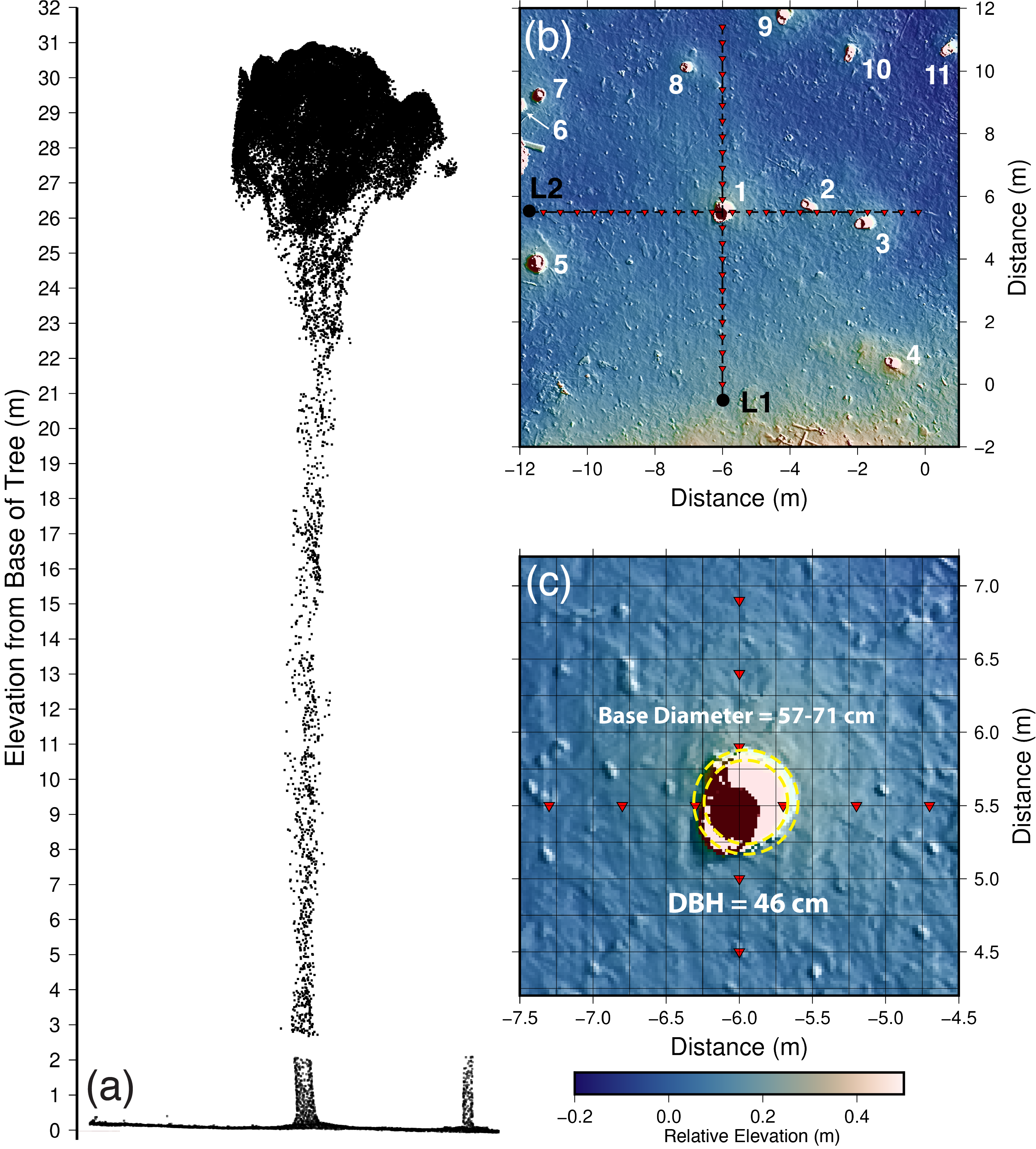
(a) Reconstructed 3D point cloud of the longleaf pine (tree #1 in panel b), viewed along profile L1. (b) High-resolution DEM of the study area (2 cm resolution). Each tree is numbered for reference. The two seismic profiles are shown as black lines, with black circles marking the start of each profile. Red inverted triangles indicate the locations of geophones. (c) Magnified view of the base of the large pine. The trunk diameter at the soil interface ranges from 57 cm to 71 cm, and the soil is visibly raised around the base.
Seismic Refraction
Two seismic refraction profiles, each 11.5 m long and oriented perpendicular to one another, were collected with the largest tree (tree #1) positioned at their intersection (Figures 1, 2). Both profiles used 24 geophones spaced at 50 cm intervals. The spacing between the 12th and 13th geophones exceeded 50 cm to accommodate the large diameter at the base of the tree (see Figures 1c, 2). Shot points were located at each geophone position. Each shot record was collected for 0.5 s with a sampling rate of 16.1 kHz. A maximum of 552 first-arrival picks was possible for each profile.
To obtain P-wave velocities (\(V_p\)), data were collected with 4.5 Hz vertical geophones and a sledgehammer striking a steel plate. Each shot in the P-wave survey was stacked four times to improve signal-to-noise. To obtain S-wave velocities (\(V_s\)), the vertical geophones were replaced with 4.5 Hz horizontal geophones oriented perpendicular to the profile (Figure 2). The profile was re-shot using a sledgehammer striking an I-beam that generated transversely polarized S-waves. Each side of the I-beam was struck and stacked four times, which produced two stacked shot records with reversed polarity.
The final gather was created by subtracting the two reversed polarity shot gathers (Uhlemann et al. 2016; Hunter et al. 2022). The reported S-wave velocities \(V_{s}\) in this study represent horizontal S-wave velocities (\(V_{sh}\)), not vertical S-wave velocities (\(V_{sv}\)).In isotropic and elastic media, Sh waves are decoupled from P-Sv waves (Stein and Wysession 2003). Therefore, Sh waves do not produce mode conversions at boundaries. Thus, the first arrivals from the S-wave surveys are interpreted as refracted Sh waves not direct or converted P-waves.
First arrivals for both P- and S-waves were picked manually and then inverted using travel-time tomography (Zelt et al. 2013; Sheehan, Doll, and Mandell 2005). Due to the short offsets, the signal-to-noise ratio was high, allowing over 90% of first arrivals to be picked without filtering. The first-arrival times were inverted using the refraction module in the Python Geophysical Inversion Modeling Library (PyGIMLi) (Rücker, Günther, and Wagner 2017). The forward model assumed elastic energy traveled as rays, computed using the shortest path algorithm (Dijkstra 1959; T. Moser 1991; T. J. Moser, Nolet, and Snieder 1992). Inversion was performed using a deterministic Gauss–Newton scheme that minimized the \(\chi^2\) error metric. Each arrival was assigned an uncertainty of 0.5 ms. All arrivals were inverted on the same triangular mesh, and identical smoothing parameters were applied to each model.
Uncertainty was estimated by inverting the first arrivals 100 times using different starting velocity models. For the P-wave inversions, the top velocity ranged from 100 to 1500 m/s, and the vertical velocity gradient ranged from 3 to 30 m/s/m. For the S-wave inversions, the top velocity ranged from 50 to 1000 m/s, with the same gradient range of 3 to 30 m/s/m. Final velocity models were computed by averaging the velocity in each cell across all 100 inversions. The root mean square errors (RMSE) were calculated by tracing rays through the model generated from the mean of the 100 inversions and can be found in the Supplemental Materials.
Each inverted model had slightly different ray coverage. To compare \(V_{p}\) and \(V_{s}\), a conservative masking procedure was applied. The mask excluded model cells that had fewer than 25 rays passing through them. For example, if a cell in the P-wave inversion was intersected by ray paths in only 24 of the 100 inversions, it was excluded from the profiles presented in the results. This conservative approach ensured that the profiles shown in the results section represent areas where \(V_{p}\), \(V_{s}\), and consequently (\(V_{p}/V_{s}\)) values were well constrained.
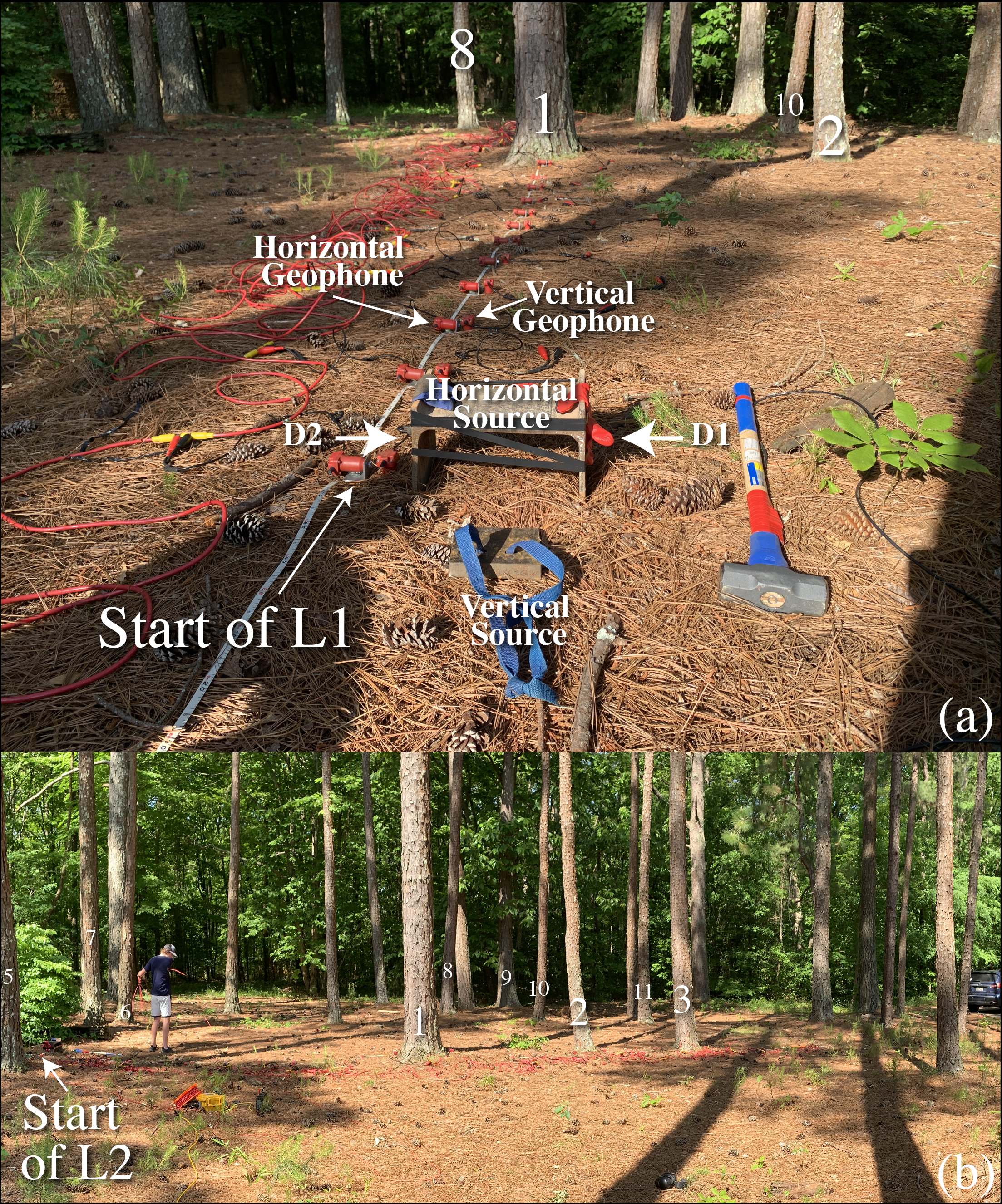
Images illustrating the collection of seismic refraction data. Tree labels correspond to those shown in Figure 1. (a) Perspective view from the beginning of profile L1. Both vertical and horizontal geophones were deployed; however, the vertical geophones were not connected due to a limited number of recording channels. The vertical source was a small steel plate, while the horizontal source was a custom-made I-beam. Directions D1 and D2 indicate the orientation of the horizontal geophones. The I-beam source minimized vertical displacements and generated transversely polarized S-waves with opposite polarity. (b) Photograph showing the full deployment of profile L2.
General Shear Failure
Like any freestanding structure, trees must overcome the force of gravity. The concept of soil bearing capacity provides a framework for interpreting the geophysical results. Soil bearing capacity defines the maximum vertical load a soil can support before deforming beyond a specified threshold. One model that describes how a solid body fails under vertical loading is the Prandtl Wedge (Figure 3) (Van Baars 2018). The Prandtl Wedge offers an analytical solution for estimating the extent of settlement beneath a footing. This model was later refined and is now a standard method for describing soil shear failure under various shapes and loading conditions (Terzaghi 1943; Meyerhof 1963; Hansen et al. 1970).
General shear failure under an applied vertical load in unconsolidated soils occurs along well-defined shear failure planes that divides the soil into three distinct zones (Figure 3). The first zone is triangular and located directly beneath the applied load, where the principal stresses are vertical. The shape of this zone is governed by the soil’s internal angle of friction (\(\phi\)). The second zone is a wedge bounded below by a logarithmic spiral. During shear failure, this wedge moves upward toward the surface, producing soil heave. The third zone is another triangular region, but here the principal stresses are horizontal, in contrast to the vertical stresses in the first zone.
The soil bearing capacity is determined by calculating the maximum load that can be applied to the soil without causing displacement, assuming failure occurs along the boundaries defined by the Prandtl Wedge (Figure 3). To construct the Prandtl Wedge, the coordinates of five key points—\(A, C, D, E,\) and \(F\)—were calculated to define the vertices of the three shear failure zones (Figure 3). The equations provided here describe only one side of the wedge, but the geometry is symmetric. Each point represents a coordinate (e.g., \(A = (A_x, A_y)\)). The shape of the wedge depends on \(\phi\) and the width (\(W\)) of the applied load. First, two angles (\(\theta_1\) and \(\theta_2\)) were calculated based on \(\phi\), such that their sum equals a right angle.
To calculate points \(A\) and \(C\), the applied load is centered at the origin and located at the surface:
Since \(\theta_1\) depends on \(\phi\), point \(D\) is derived using trigonometric relationships:
Next, the length \(r_1\) is calculated as follows:
To calculate the length of \(r_3\) the equation for a logarithmic spiral is used:
Then, the length of \(r_3\) is used to calculate the Cartesian coordinates of point \(E\):
Point \(F\) is twice the distance of \(E_x\) and is located on the surface:
To visualize the slip plane that defines the bottom of zone three, the logarithmic spiral for the angle spanned by the vector connections \(\overline{CD}\) and \(\overline{CE}\) is calculated as follows:
The radial values of \(r_2\) were transformed into Cartesian coordinates:
The logarithmic spiral is a parametric equation that defines the radial length of the wedge. To align \(r_2\) with points \(D\) and \(E\) the spiral must be rotated by the angle \(\alpha\):
Finally, the rotation was transformed into Cartesian coordinates as follows:
Thus, \(r_{xx}\) and \(r_{yy}\) define the bottom of the wedge that defines zone two (blue lines in Figure 3). To plot the other side of the wedge, the x-coordinates were multiplied by negative one to reflect them over the y-axis. A summary of the derivation can be found in (Van Baars 2018).
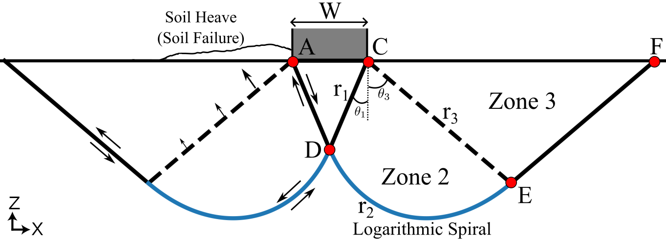
General shear failure as depicted by the Prandtl Wedge. Zone 1 is the triangular region directly beneath the applied load. Zones 2 and 3 are labeled accordingly. On the left side of the wedge, arrows indicate the direction of material movement along the slip planes. The arrows along the dashed line show that Zone 2 moves upward toward the surface after failure, resulting in soil heave near the point of loading.
Results
The P- and S-wave data produced clear and continuous first arrivals. The S-wave arrivals were always delayed relative to P-wave arrivals. The subtraction opposite polarity shots generated by the I-beam increased the signal-to-noise of the first arrivals for the S-wave surveys. Examples of shot gathers, picked arrivals, and RMSE misfits for the inversions are provided in the Supplemental Material.
Along L1, tree #1 was located between 4.5 and 5.5 m. Tree #8 was located between 9.5 and 10.5 m. Tree #8 was one of the smaller trees in the stand (DBH = 24 cm) and was offset from the profile by 1̃ m (Figure 4a–c). Along L2, tree #1 was located between -6.5 and 5.5 m. Tree #2 was located between -4 and -3 m. Tree #3 was located between -2 and -1 m. Both tree #2 and #3 were offset from the profile. Tree #3 was larger than tree #2 with a DBH of 35 cm. Tree #2 was the smallest in the stand with a DBH of 22 cm.
The \(V_{p}\) profile along L1 showed localized zones of lower velocities (\(V_{p} \le 375\) m/s). These low velocity zones occurred on both sides of tree #1 (Figure 4b). The \(V_{s}\) profile had similar structure to the \(V_{p}\), which included the localized low velocity zones (\(V_{s} \le 200\) m/s)on each side of tree #1 (Figure 4a). However, unlike the \(V_{p}\) profile, the \(V_{s}\) profile revealed a high-velocity anomaly (\(V_{s} \ge 350\) m/s) below the tree. The high-velocity anomaly was approximately 1 to 1.5 m wide and extended to depths greater than 1.5 m (Figure 4a).
The \(V_{p}\) profile along L2 appeared asymmetrical. From -12 to -6 m, the \(V_{p}\) profile was dominated by low velocities (\(V_{p} \le 375\) m/s) (Figure 4e). Around -6 m, a region of higher velocities (\(V_{p} \ge 500\) m/s) appeared at elevations less than -1 m. These higher \(V_p\) approached the surface under tree #3, where \(V_{p}\) was greater than 500 m/s. The \(V_{s}\) profile had a similar asymmetrical structure to the \(V_{p}\), with lower velocities (\(V_{s} \le 200\) m/s) from -12 to - 6 m and higher velocities (\(V_{s} \ge 350\) m/s) that approached the surface under tree #3. However, unlike the \(V_{p}\) profile, the \(V_{s}\) profile showed a high-velocity anomaly (\(V_{s} \ge 350\) m/s) below tree #1. This high-velocity anomaly had a similar shape to the anomaly under L1.
Both L1 and L2 revealed low \(V_{p}\)/\(V_{s}\) values (<1.5) under tree #1 (Figure 4c,f). These low \(V_{p}\)/\(V_{s}\) values were driven by \(V_{s}\). A similar low \(V_{p}\)/\(V_{s}\) anomaly occurred under tree #3 along L2 and appeared at the start of L1 between 0 and 1.5 m (Figure 4c). Low \(V_{p}\)/\(V_{s}\) values were not visible under trees #8 on L1 and #2 on L2. The \(V_{p}\)/\(V_{s}\) values were higher (> 1.8) near the surface on either side of tree #1 (4c,f). The \(V_{p}\)/\(V_{s}\) values of both profiles matched well at the intersection (Figure 5). An Interactive . html file of Figure 5 is provided in the Supplemental Material (Dropbox link for now).
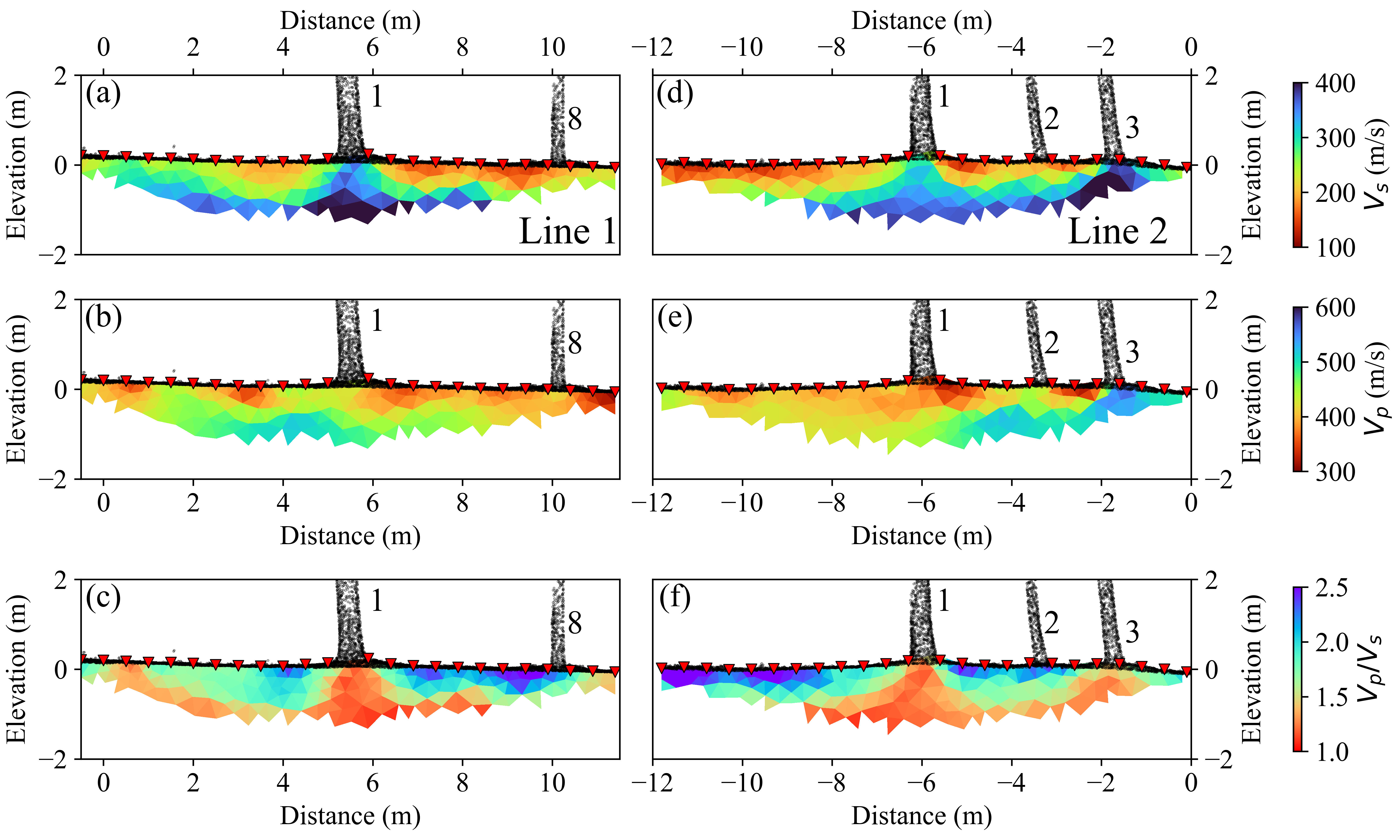
\(V_s\), \(V_p\), and \(V_p/V_s\) values for profiles L1 and L2, shown without vertical exaggeration. X-axis distances correspond to the local coordinate system in Figure 1b. The above-ground structure is a 3D point cloud generated via SfM, highlighting tree locations. Trees are labeled. Only tree #1 passes directly through both profiles. Inverted red triangles indicate geophone positions. The top row (panels a and b) displays S-wave velocity profiles; the middle row (panels c and d) shows P-wave velocity profiles; and the bottom row (panels e and f) presents \(V_p/V_s\) values.
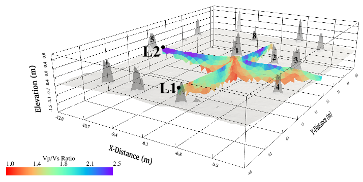
A 3D perspective of the \(V_{p}/V_{s}\) values along L1 and L2, shown without vertical exaggeration. The DEM is plotted over the profiles to indicate tree locations. The start of each profile is labeled and marked with a black dot. An interactive .html file is available for download here.
Discussion
Data from two 11.5 m perpendicular \(V_{p}\) and \(V_{s}\) profiles, intersecting beneath a 31 m tall longleaf pine, were presented (Figure 1). High-velocity \(V_{s}\) anomalies were observed beneath trees #1 and #3 (Figure 4). The \(V_{p}/V_{s}\) values remained consistent between the two profiles and matched at the intersection (Figure 5). The low \(V_{p}/V_{s}\) values were caused by changes in \(V_{s}\) beneath trees #1 and #3 (Figures 4 and 5).
The shape of the \(V_s\) and \(V_{p}/V_{s}\) values, specifically the width, depth, and triangular form of the anomalies beneath tree #1, resembled the failure planes defined by the Prandtl wedge (Figure 3 versus Figure 4). To explore the structural similarities, I will focus on the \(V_{p}/V_{s}\) profiles. To compare, the seismic data were transformed from elevation to depth, and each profile was shifted to place tree #1 at the origin.
To compare, shear failure planes were calculated assuming \(\phi = 28^{\circ}\), a typical value for Piedmont soils (Borden, Shao, and Gupta 1996; Murdoch et al. 2006). The width of the footing was set to 66 cm to match the average diameter at the base of tree #1 (Figure 1). The three zones of the Prandtl wedge were computed using Equations [eq:wedge_first] to [eq:wedge_final] and then superimposed on the \(V_{p}/V_{s}\) values from L1 and L2 (Figure 6).
The \(V_{p}/V_{s}\) values located in each of the three Prandtl wedge zones were extracted for statistical analysis (Figure 6c). The distributions included \(V_{p}/V_{s}\) values from L1 and L2. The mean and standard errors for each zone were: Zone one—\(1.25 \pm 0.02\) (N=8), Zone two—\(1.45 \pm 0.02\) (N=66), and Zone three—\(2.02 \pm 0.02\) (N=101). These three distributions had statistically distinct means (\(p < 0.05\)) (Figure 6c). The means remained statistically significant even when the internal friction angles varied from 20° and 31° (see Supplemental Material). Thus, the lowest \(V_{p}/V_{s}\) values, were associated with the highest \(V_{s}\) values and occurred in regions where the largest displacements under a simple model describing normal shear failure are expected. These observations, which bridge concepts from seismology and soil mechanics, suggest the following hypothesis: trees opportunistically grow vertically oriented roots along shear failure planes predicted by basic soil mechanics.
Central to this hypothesis are two potential mechanisms that could explain the increase in \(V_{s}\) directly beneath the tree. The first is that vertically oriented roots beneath the tree may like soil nails or rebars in concrete. By intersecting the potential shear failure plane, they increase cohesion along the slip surfaces they cross. The degree of strengthening would depend on the angle at which the roots intersect these planes. This mechanism is consistent with existing literature that shows roots increase the soil cohesion (Ali and Osman 2008; Jian et al. 2024; Ghestem et al. 2014).
The second mechanism is that the weight of the tree induced localized shear strains over time. These strains caused grains to interlock along failure planes, which increased the shear modulus. Thus, the \(V_{s}\) represents a snapshot in time. This may seem counter-intuitive from a geophysical perspective because the elastic moduli are assumed to be a static material property. However, in soil mechanics, it is well known that the mechanical response of a soil will depend on its stress history. The stress history of a material is quantified using the overconsolidation ratio (OCR) (Atkinson 2007; Rajapakse 2015).
Thus, it is critical to understand the connection between the shear failure envelope (Figure 3 and Equations [eq:wedge_first]–[eq:wedge_final]) and the \(V_s\) velocities measured using seismic refraction (Figure 4). The shear failure planes (Figure 6a,b; and Figure 3) were derived using a simplified model that assumed the weight of the tree was uniformly distributed at the soil interface. Under these assumptions, the failure planes in Figure 3 develop when the downward stress exerted by the tree exceeds the shear strength of the soil. In other words, the Prandtl Wedge makes a prediction about where the ground will permanently deform under large loads that exceed the maximum shear strength of the soil.
In contrast, the \(V_{p}/V_{s}\) values estimated using seismic refraction assume that the soil behaves as an elastic material. This means there is never permanent deformation. The assumption of linear elasticity is appropriate for seismic waves, which induce small strains on the order of \(10^{-5}\) to \(10^{-6}\) (Cheng and Johnston 1981; Ng, Pun, and Pang 2000; Kung 2010). This is why the comparison shown in Figure 6 is not apples-to-apples. Figure 6 compares a prediction where deformation will occur under large strains (\(10^{-2}\) to \(10^{0}\) ) with the elastic response at small strains where no permenant deformation will occur. The seismic observations are a snapshot in time, which includes the material’s deformation history caused by the increasing stresses as the tree grows. In other words, the seismic data are sensitive to the material’s dynamic modulus and not a direct measurement of the shear strength of the soil.
Shear strength and dynamic shear modulus are not the same, but they are related. Shear strength refers to the maximum stress a material can withstand before undergoing permanent deformation. In contrast, the shear modulus is defined as the ratio of shear stress (\(\tau\)) to shear strain (\(\gamma\)), representing the material’s stiffness under elastic deformation.
In other words, \(G\) describes the material’s ability to resist shear deformation when a shear stress is applied. If the applied stresses and strains are small, it is reasonable to assume that the material will behave in a linear and elastic manner. This assumption is inherent in the construction of the \(V_p\) and \(V_s\) profiles (Figure 4).
Understanding how a material responds to larger stresses and strains is critical for evaluating soil failure. A theoretical stress–strain curve from a direct shear test is shown in Figure 7a. This curve represents the typical response of soil during such a test. In a direct shear test, soil is placed in a small box, and shear stresses are applied to induce a predictable failure plane along the center of the sample (Gan, Fredlund, and Rahardjo 1988). This characteristic curve illustrates how soil responds across a wide range of stresses and strains (Figure 7a). The curve in Figure 7 was sketched based on general trends observed in direct shear tests conducted on soils with and without roots (Ali and Osman 2008; Jian et al. 2024; Ghestem et al. 2014). Numerical values were omitted to emphasize the curve’s shape—particularly the increase in peak strength due to root presence—and to highlight how this behavior relates to the \(V_s\) profiles shown in Figure 4a,b.
The stress–strain curve (Figure 7a) is related to \(V_s\) through the shear modulus \(G\) (Equation [eq:G]). In a linear elastic framework, which is assumed for seismic wave propagation, \(G\) is a material property that determines the amount of strain produced by a given stress. In the theoretical stress–strain curve, the shear modulus is illustrated by colored straight-line segments, representing the slope in this domain (see Equation [eq:G]). Under small strains, these segments provide a good approximation of the material’s response. However, as stresses and strains increase, the mechanical behavior deviates from linearity, and a straight line no longer describes the response—particularly beyond the peak shear strength \(\tau\) (Figure 7a).
Thus, the relationship between the shear modulus at different strain values is described by the shear modulus reduction curve (Figure 7b). The modulus reduction curve can be generated from the direct shear test by calculating the shear modulus (stress divided by strain) at every point along the curve and normalizing it using the dynamic shear modulus \(G_0\):
The normalized shear modulus is plotted against strain, which is also normalized by the reference strain calculated by dividing the peak shear strength by \(G_0\). This curve is typically shown on a log-linear scale to emphasize the significant reduction in shear modulus as strain increases (Figure 7b). For linear elastic and isotropic systems, Equation [eq:G0] is also referred to in seismology as the shear modulus, with units of pressure, typically expressed in MPa or GPa. In seismology, \(G_0\) is often treated as a constant material property. However, from a soil mechanics perspective, \(G\) depends on the stress.
Although \(G_0\) can be estimated using an assumed soil density of 1600 kg/m3 (Figure 7c,d), these values are significantly higher than those typically used in soil mechanics or geotechnical modeling. This discrepancy arises because buildings or foundations often load the soil beyond the elastic range, where \(G\) is no longer valid. Nevertheless, \(G_0\) represents the maximum shear modulus, and the modulus reduction curve relates \(G_0\) to the shear modulus at the expected strain level (Figure 7b).
Tree #1 was still growing, which indicates that no major shear failure occurred. However, the slightly elevated topography around its base, and around other trees in the area, may suggest displacement along the shear failure envelope during the tree’s growth. This process is analogous to pressing an object into loose, dry sand, where displaced sand forms a raised ridge around the depression. Similar raised ridges were visible in the high-resolution DEM around the larger trees in the study area (Figures 1 and 2).
As the tree grew, its increasing mass exerted a greater downward force. Eventually, the tree’s weight exceeded the soil’s bearing capacity, and the soil failed. In this context, “failure” refers to soil movement, as bearing capacity is defined as the maximum load the soil can support without displacement. The failure was not catastrophic—it was not large enough to cause the tree to topple. The raised rings observed around most of the larger trees in the study area are interpreted as evidence of soil heave (Figure 1). These raised rings might explain why there were low \(V_{p}/V_{s}\) values observed under tree #3, which has a larger ring, and not tree #2 and #8 (Figure 1b). The larger trees a few meters away from the start of L1 (see Figure 5). These trees also produced raised rings that are visible in at the start of Figure 1b.
Tree #1 was not cored, so its age remains unknown. However, based on its height, the tree is likely between 30 and 50 years old. Unlike civil infrastructure, which is designed to minimize settlement due to shear failure, a tree can “fail” in the traditional engineering sense as it grows. If the soil beneath the tree fails along defined shear planes, the tree may only need to reinforce a small region directly beneath its trunk. Alternatively, if strain has already accumulated along the shear failure plane, the resulting seismic survey could image the shear strengthening effect caused by the tree’s weight. These results were unexpected; therefore, we did not core or remove the tree. Additional geotechnical investigations are needed to distinguish between these two possible mechanisms.
From a seismological perspective, the observed \(V_{p}/V_{s}\) values are significantly lower than expected and warrant further investigation. \(V_{p}/V_{s}\) values below 1.4 are uncommon in rocks and should be interpreted with caution (Mavko, Mukerji, and Dvorkin 2009). In perfectly elastic and isotropic materials, \(V_{p}/V_{s}\) values less than or equal to \(\sqrt{2} \approx 1.4\) result in a negative Poisson’s ratio. Materials with negative Poisson’s ratios behave counterintuitively, contracting laterally when compressed (Acuna et al. 2022; Alderson and Alderson 2007; Evans and Alderson 2000; Ji et al. 2018; Ji, Wang, and Li 2019). In this study, low \(V_{p}/V_{s}\) values were observed exclusively beneath the tree (Figure 5). The mean \(V_{p}/V_{s}\) value derived from both profiles was 1.6, which is consistent with values reported for dense to loose sands (Thota, Cao, and Vahedifard 2021).
\(V_{p}/V_{s}\) values below 1.4 have previously been documented in shallow subsurface environments under low confining pressures (B. A. Flinchum et al. 2024; Trichandi et al. 2022; Liu, Zhu, and Hayes 2022). It is unlikely that the observed \(V_{p}/V_{s}\) values below 1.4 are inversion artifacts for two reasons. First, the velocity models did not exhibit large velocity contrasts that would have produced reflections or converted phases. Second, the maximum offset was only 11.5 m, which minimized the space required for phases to separate. Furthermore, the low \(V_{p}/V_{s}\) values appeared as localized yet continuous structures. If these values were inversion artifacts, they would have occurred near strong velocity gradients, which were not observed.
Thus, the final interpretation is that the roots, or displacements along failure planes caused shear strengthening. Both of these would create an increase in \(V_s\). However, the lack of a clear \(V_p\) under the tree suggest that the cracks or pore spaces beneath the tree were not fully closed; otherwise, there would have been significant increase in \(V_p\) (Berryman, Pride, and Wang 2002; Holbrook et al. 2014; Budiansky and Oconnell 1976). This would have resulted in higher \(V_{p}/V_{s}\) values. For example, in larger trees such as the giant redwoods, sequoias, or eucalyptus trees in Tasmania, the weight may be sufficient to compress the soil, reduce porosity, and increase the \(V_{p}/V_{s}\) values beneath the tree.
The data and discussion provided suggest that further testing is needed, particularly cross-disciplinary work between near-surface geophysicists and geotechnical engineers. The observations also suggest that it is possible to extract more than just structural information from \(V_p\) and \(V_s\). Furthermore, seismic refraction can be a valuable tool for studying the hidden and difficult-to-access root systems that support trees.
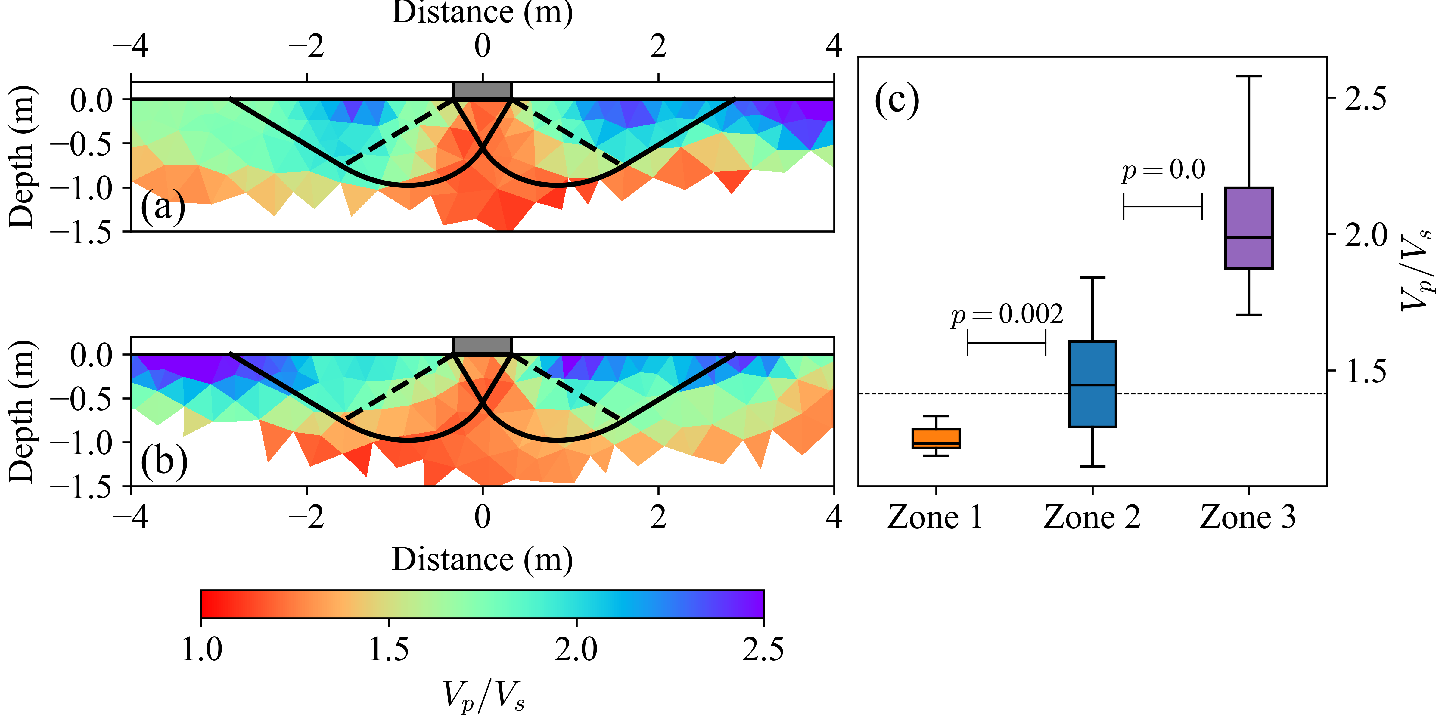
Comparison between the predicted shear failure planes from the Prandtl-wedge model and the \({V_s}\) profiles for (a) L1 and (b) L2. The Prandtl-wedge was calculated using an internal friction angle of \(28^{\circ}\) (\(\phi = 28^{\circ}\)). The \(V_s\) profiles were converted from elevation to depth and translated such that tree #1 is located at the origin. Additionally, the velocity profile for L2 was increased by 10%. (c) Box plots of \(V_p/V_s\) values within the wedge zones shown in panels (a) and (b). The boxes represent the first (Q1) and third (Q3) quartiles, with the black line indicating the median. Whiskers extend to 1.5 times the interquartile range (IQR). The thin horizontal dashed line marks a \(V_p/V_s\) value of \(\sqrt{2}\). Changes in \(V_p/V_s\) values are driven by variations in \(V_s\), as \(V_p\) remained relatively constant.
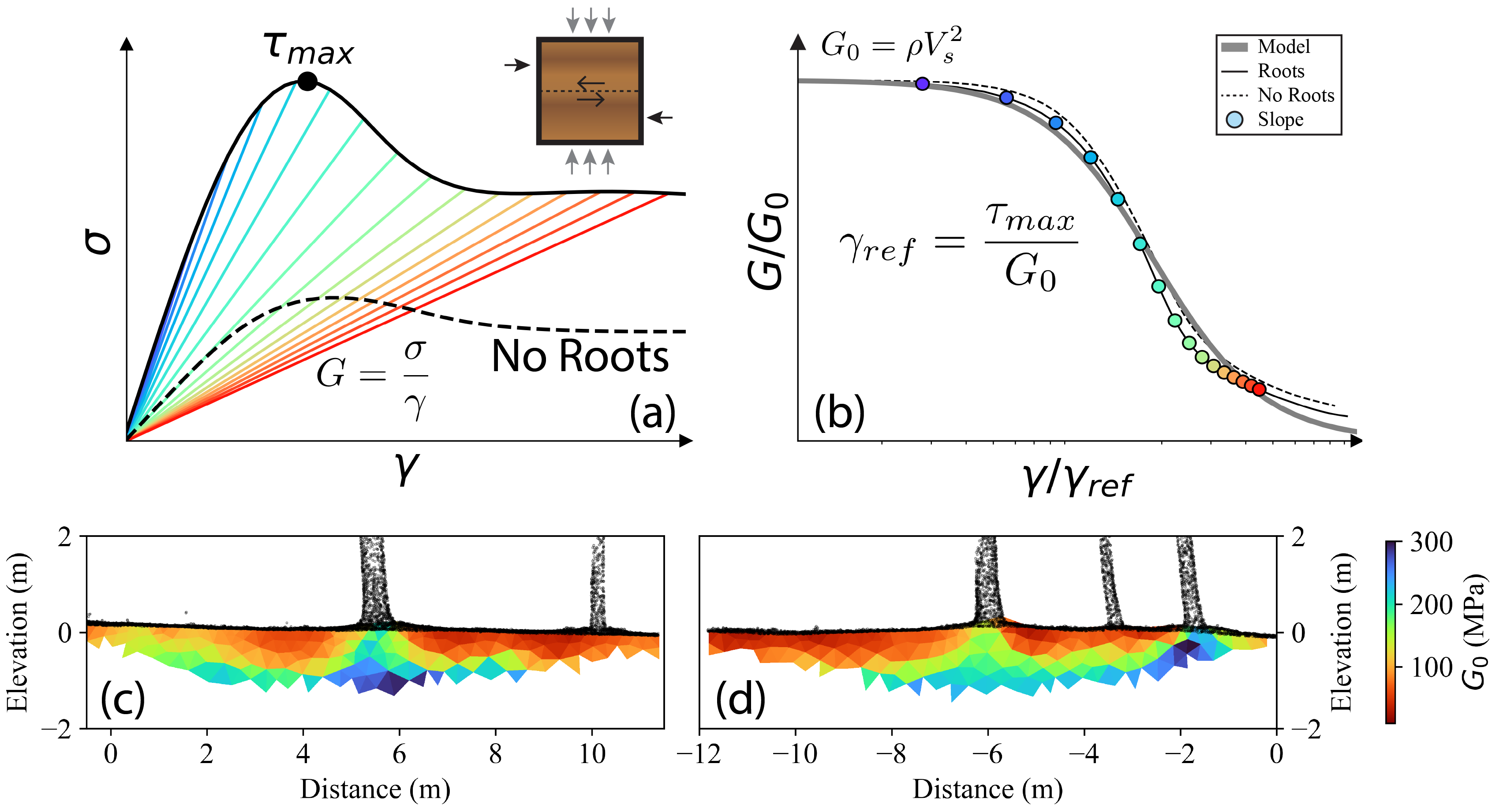
(a) An example of a direct shear test illustrating how the shear modulus (\(G\)) changes with increasing strain. The shear modulus remains relatively constant up to the maximum shear stress, then rapidly decreases after the peak shear stress (\(\tau_{max}\)) is reached. The upper right inset shows the shear failure plane developed during the test. (b) A shear modulus reduction curve relating the shear modulus, normalized by the small-strain stiffness (\(G_0\)), to the normalized strain. Colored dots correspond to different slopes in panel (a). The thick gray line represents a standard model, while the thin and dashed black lines correspond to the curves from panel (a). (c) \(G_0\) calculated for L1, assuming a soil density of 1600 kg/m3. (d) \(G_0\) calculated for L2, also assuming a soil density of 1600 kg/m3.
Conclusion
The data presented here demonstrate the applicability of high-resolution seismic refraction surveys as a novel tool for investigating the relationship between tree root structures and soil mechanical properties. By analyzing P-wave and horizontally polarized S-wave velocities around a 31 m tall longleaf pine in the South Carolina Botanical Gardens, minimal changes in \(V_p\) were observed, while \(V_s\) increased, resulting in low \(V_{p}/V_{s}\) values directly beneath the tree. These findings suggest that vertical roots enhance soil shear strength while preserving porosity and compressibility. The alignment of the observed \(V_{p}/V_{s}\) structure with the predicted shear failure envelope implies that trees may opportunistically grow roots to reinforce soil along shear failure planes. This research underscores the importance of root–soil interactions and introduces a non-invasive method for evaluating the mechanical influence of roots on soil stability. These insights could have broad implications for forestry, agriculture, and environmental conservation. Future studies should prioritize interdisciplinary collaborations to validate these findings across diverse tree species and environmental settings.
Acknowledgements
I am grateful to Jonathan Cochran, an undergraduate student, for his assistance in collecting the seismic refraction data as part of his senior research project. I sincerely thank Dr. N. (Ravi) Ravichandran for initiating discussions on tree roots and foundations, and for many engaging conversations on fundamental soil mechanics. I also appreciate Dr. Don Hagan for numerous insightful discussions about trees and their root systems. Special thanks to my colleague George Kouretzis for reviewing this manuscript prior to submission. As a geophysicist and critical zone scientist, I approached the geotechnical aspects of this work with some trepidation, and his feedback was invaluable. I am also thankful for the many conversations over the years that have shaped my thinking about making the critical zone more accessible. I am also thankful for the two reviewers who provided excellent suggestions to improve this manuscript. This study was supported by Clemson University.
Abe, Kazutoki, and Robert R. Ziemer. 1991. “Effect of tree roots on a shear zone: modeling reinforced shear stress.” Canadian Journal of Forest Research 21 (7): 1012–19. https://doi.org/10.1139/x91-139.
Acuna, Daniel, Francisco Gutiérrez, Rodrigo Silva, Humberto Palza, Alvaro S. Nunez, and Gustavo Düring. 2022. “A three step recipe for designing auxetic materials on demand.” Communications Physics 5 (1): 113. https://doi.org/10.1038/s42005-022-00876-5.
Alderson, A, and K L Alderson. 2007. “Auxetic materials.” Proceedings of the Institution of Mechanical Engineers, Part G: Journal of Aerospace Engineering 221 (4): 565–75. https://doi.org/10.1243/09544100jaero185.
Ali, Faisal Haji, and Normaniza Osman. 2008. “Shear Strength of a Soil Containing Vegetation Roots.” Soils and Foundations 48 (4): 587–96. https://doi.org/10.3208/sandf.48.587.
Ancelin, Philippe, Benoît Courbaud, and Thierry Fourcaud. 2004. “Development of an individual tree-based mechanical model to predict wind damage within forest stands.” Forest Ecology and Management 203 (1-3): 101–21. https://doi.org/10.1016/j.foreco.2004.07.067.
Atkinson, John. 2007. The Mechanics of Soils and Foundations. Milton, UNITED KINGDOM: Taylor & Francis Group. http://ebookcentral.proquest.com/lib/newcastle/detail.action?docID=308681.
Befus, K. M., A. F. Sheehan, M. Leopold, S. P. Anderson, and R. S. Anderson. 2011. “Seismic Constraints on Critical Zone Architecture, Boulder Creek Watershed, Front Range, Colorado.” Vadose Zone Journal 10 (4): 1342–42. https://doi.org/10.2136/vzj2010.0108er.
Berryman, James G, Steven R Pride, and Herbert F Wang. 2002. “A Differential Scheme for Elastic Properties of Rocks with Dry or Saturated Cracks.” Geophysical Journal International 151 (2): 597–611. https://doi.org/10.1046/j.1365-246x.2002.01801.x.
Borden, Roy H, Lisheng Shao, and Ayushman Gupta. 1996. “Dynamic Properties of Piedmont Residual Soils.” Journal of Geotechnical Engineering 122 (10): 813–21. https://doi.org/10.1061/(asce)0733-9410(1996)122:10(813).
Brantley, S. L., J. P. Megonigal, F. N. Scatena, Z. Balogh-Brunstad, R. T. Barnes, M. A. Bruns, P. Van Cappellen, et al. 2011. “Twelve testable hypotheses on the geobiology of weathering.” Geobiology 9 (2). https://doi.org/10.1111/j.1472-4669.2010.00264.x.
Budiansky, B., and Rj Oconnell. 1976. “Elastic-Moduli of a Cracked Solid.” International Journal of Solids and Structures 12 (2): 81–97. https://doi.org/10.1016/0020-7683(76)90044-5.
Butnor, J. R., J. A. Doolittle, L. Kress, S. Cohen, and K. H. Johnsen. 2001. “Use of ground-penetrating radar to study tree roots in the southeastern United States.” Tree Physiology 21 (17): 1269–78. https://doi.org/10.1093/treephys/21.17.1269.
Canadell, J., R. B. Jackson, J. B. Ehleringer, H. A. Mooney, O. E. Sala, and E.-D. Schulze. 1996. “Maximum rooting depth of vegetation types at the global scale.” Oecologia 108 (4): 583–95. https://doi.org/10.1007/bf00329030.
Cheng, C. H., and David H. Johnston. 1981. “Dynamic and Static Moduli.” Geophysical Research Letters 8 (1): 39–42. https://doi.org/10.1029/gl008i001p00039.
Currey, Donald R. 1965. “An Ancient Bristlecone Pine Stand in Eastern Nevada.” Ecology 46 (4): 564–66. https://doi.org/10.2307/1934900.
Danjon, Frédéric, Thierry Fourcaud, and Didier Bert. 2005. “Root architecture and wind‐firmness of mature Pinus pinaster.” New Phytologist 168 (2): 387–400. https://doi.org/10.1111/j.1469-8137.2005.01497.x.
Dijkstra, E. W. 1959. “A note on two problems in connexion with graphs.” Numerische Mathematik 1 (1): 269–71. https://doi.org/10.1007/bf01386390.
Docker, B. B., and T. C. T. Hubble. 2008. “Quantifying Root-Reinforcement of River Bank Soils by Four Australian Tree Species.” Geomorphology 100 (3-4): 401–18. https://doi.org/10.1016/j.geomorph.2008.01.009.
Dumroese, R. Kasten, Mattia Terzaghi, Donato Chiatante, Gabriella S. Scippa, Bruno Lasserre, and Antonio Montagnoli. 2019. “Functional Traits of Pinus ponderosa Coarse Roots in Response to Slope Conditions.” Frontiers in Plant Science 10: 947. https://doi.org/10.3389/fpls.2019.00947.
Dupuy, Lionel X., Thierry Fourcaud, Patrick Lac, and Alexia Stokes. 2007. “A generic 3D finite element model of tree anchorage integrating soil mechanics and real root system architecture.” American Journal of Botany 94 (9): 1506–14. https://doi.org/10.3732/ajb.94.9.1506.
Ehosioke, Solomon, Frédéric Nguyen, Sathyanarayan Rao, Thomas Kremer, Edmundo Placencia‐Gomez, Johan Alexander Huisman, Andreas Kemna, Mathieu Javaux, and Sarah Garré. 2020. “Sensing the Electrical Properties of Roots: A Review.” Vadose Zone Journal 19 (1). https://doi.org/10.1002/vzj2.20082.
Evans, K E, and K L Alderson. 2000. “Auxetic materials: the positive side of being negative.” Engineering Science & Education Journal 9 (4): 148–54. https://doi.org/10.1049/esej:20000402.
Flinchum, B. A., D. Grana, B. J. Carr, N. Ravichandran, B. Eppinger, and W. S. Holbrook. 2024. “Low Vp/Vs Values as an Indicator for Fractures in the Critical Zone.” Geophysical Research Letters 51 (2). https://doi.org/10.1029/2023gl105946.
Flinchum, Brady A., W. Steven Holbrook, Daniella Rempe, Seulgi Moon, Clifford S. Riebe, Bradley J. Carr, Jorden L. Hayes, James St. Clair, and Marc Philipp Peters. 2018. “Critical Zone Structure Under a Granite Ridge Inferred From Drilling and Three‐Dimensional Seismic Refraction Data.” Journal of Geophysical Research: Earth Surface 123 (6): 1317–43. https://doi.org/10.1029/2017jf004280.
Gan, J. K. M., D. G. Fredlund, and H. Rahardjo. 1988. “Determination of the Shear Strength Parameters of an Unsaturated Soil Using the Direct Shear Test.” Canadian Geotechnical Journal 25 (3): 500–510. https://doi.org/10.1139/t88-055.
Ghestem, Murielle, Guillaume Veylon, Alain Bernard, Quentin Vanel, and Alexia Stokes. 2014. “Influence of plant root system morphology and architectural traits on soil shear resistance.” Plant and Soil 377 (1-2): 43–61. https://doi.org/10.1007/s11104-012-1572-1.
Giadrossich, F., M. Schwarz, D. Cohen, A. Cislaghi, C. Vergani, T. Hubble, C. Phillips, and A. Stokes. 2017. “Methods to measure the mechanical behaviour of tree roots: A review.” Ecological Engineering 109: 256–71. https://doi.org/10.1016/j.ecoleng.2017.08.032.
Guo, Li, Jin Chen, Xihong Cui, Bihang Fan, and Henry Lin. 2013. “Application of ground penetrating radar for coarse root detection and quantification: a review.” Plant and Soil 362 (1-2): 1–23. https://doi.org/10.1007/s11104-012-1455-5.
Hansen, J. Brinch, J. Brinch, Hansen bullet, and Ses nan. 1970. “A Revised and Extended Formula for Bearing Capacity.” In. https://api.semanticscholar.org/CorpusID:127983665.
Hickey, John, Parry Kostoglou, and Graham Sargison. 2000. “Tasmania’s tallest trees.” Tasforests 12 (January): 105–22.
Holbrook, W. Steven, Clifford S. Riebe, Mehrez Elwaseif, Jorden L. Hayes, Kyle Basler‐Reeder, Dennis L. Harry, Armen Malazian, Anthony Dosseto, Peter C. Hartsough, and Jan W. Hopmans. 2014. “Geophysical constraints on deep weathering and water storage potential in the Southern Sierra Critical Zone Observatory.” Earth Surface Processes and Landforms 39 (3): 366–80. https://doi.org/10.1002/esp.3502.
Hruska, Jiri, Jan Čermák, and Svatopluk Šustek. 1999. “Mapping tree root systems with ground-penetrating radar.” Tree Physiology 19 (2): 125–30. https://doi.org/10.1093/treephys/19.2.125.
Hunter, James A., Heather L. Crow, William J. Stephenson, André J.-M. Pugin, Robert A. Williams, James B. Harris, Jack K. Odum, and Edward W. Woolery. 2022. “Seismic site characterization with shear wave (SH) reflection and refraction methods.” Journal of Seismology. https://doi.org/10.1007/s10950-021-10042-z.
Jackson, R. B., J. Canadell, J. R. Ehleringer, H. A. Mooney, O. E. Sala, and E. D. Schulze. 1996. “A global analysis of root distributions for terrestrial biomes.” Oecologia 108 (3): 389–411. https://doi.org/10.1007/bf00333714.
Ji, Shaocheng, Le Li, Hem Bahadur Motra, Frank Wuttke, Shengsi Sun, Katsuyoshi Michibayashi, and Matthew H. Salisbury. 2018. “Poisson’s Ratio and Auxetic Properties of Natural Rocks.” Journal of Geophysical Research: Solid Earth 123 (2): 1161–85. https://doi.org/10.1002/2017jb014606.
Ji, Shaocheng, Qin Wang, and Le Li. 2019. “Seismic velocities, Poisson’s ratios and potential auxetic behavior of volcanic rocks.” Tectonophysics 766: 270–82. https://doi.org/10.1016/j.tecto.2019.06.013.
Jian, Shengqi, Yixue Niu, Xueli Zhang, Yi Wei, and Jun Gao. 2024. “Study on Shear Strength of Soil–Root Systems of Different Vegetation Types.” Plants 13 (21): 2963. https://doi.org/10.3390/plants13212963.
Kevern, T. C., and Arnel R. Hallauer. 1983. “Relation of Verital Root-Pull Resistance and Flowering in Maize.” Crop Science 23 (2): cropsci1983.0011183X002300020041x. https://doi.org/https://doi.org/10.2135/cropsci1983.0011183X002300020041x.
Kung, Gordon Tung-Chin. 2010. “Finite Element Analysis.” https://doi.org/10.5772/10234.
Labuz, Joseph F., and Arno Zang. 2012. “Mohr–Coulomb Failure Criterion.” Rock Mechanics and Rock Engineering 45 (6): 975–79. https://doi.org/10.1007/s00603-012-0281-7.
Li, Xinyue, Kai Jin, Peng Qin, Chunxia Liu, Xiuzhi Zhu, Yuyang Zhang, and Quanli Zong. 2024. “Enhancement Effect of Phragmites australis Roots on Soil Shear Strength in the Yellow River Delta.” Sustainability 16 (23): 10657. https://doi.org/10.3390/su162310657.
Liu, Xuejian, Tieyuan Zhu, and Jorden Hayes. 2022. “Critical Zone Structure by Elastic Full Waveform Inversion of Seismic Refractions in a Sandstone Catchment, Central Pennsylvania, USA.” Journal of Geophysical Research: Solid Earth 127 (3). https://doi.org/10.1029/2021jb023321.
Lowe, D. G. 1999. “Object Recognition from Local Scale-Invariant Features.” In Proceedings of the Seventh IEEE International Conference on Computer Vision, 2:1150–1157 vol.2. https://doi.org/10.1109/ICCV.1999.790410.
Mavko, Gary, Tapan Mukerji, and Jack Dvorkin. 2009. “The Rock Physics Handbook,” 21–80. https://doi.org/10.1017/cbo9780511626753.003.
Meyerhof, George Geoffrey. 1963. “Some Recent Research on the Bearing Capacity of Foundations.” Canadian Geotechnical Journal 1 (1): 16–26. https://doi.org/10.1139/t63-003.
Micheletti, Natan, Jim H Chandler, and Stuart N Lane. 2015. “Structure from Motion (SfM) Photogrammetry.” Geomorphological Techniques, January, 12.
Mickovski, Slobodan B., and A. Roland Ennos. 2002. “A Morphological and Mechanical Study of the Root Systems of Suppressed Crown Scots Pine Pinus Sylvestris.” Trees 16 (4): 274–80. https://doi.org/10.1007/s00468-002-0177-3.
Miller, Ashley T, H Lee Allen, and Chris A Maier. 2006. “Quantifying the coarse-root biomass of intensively managed loblolly pine plantations.” Canadian Journal of Forest Research 36 (1): 12–22. https://doi.org/10.1139/x05-229.
Montagnoli, Antonio, Mattia Terzaghi, Donato Chiatante, Gabriella S. Scippa, Bruno Lasserre, and R. Kasten Dumroese. 2019. “Ongoing modifications to root system architecture of Pinus ponderosa growing on a sloped site revealed by tree-ring analysis.” Dendrochronologia 58: 125650. https://doi.org/10.1016/j.dendro.2019.125650.
Moser, T. J., G. Nolet, and R. Snieder. 1992. “Ray bending revisited.” Bulletin of the Seismological Society of America 82 (1): 259–88. http://www.bssaonline.org/content/82/1/259.short.
Moser, Tj. 1991. “Shortest-Path Calculation of Seismic Rays.” Geophysics 56 (1): 59–67. https://doi.org/10.1190/1.1442958.
Murdoch, Lawrence C, James R Richardson, Qingfeng Tan, Shaun C Malin, and Cedric Fairbanks. 2006. “Forms and sand transport in shallow hydraulic fractures in residual soil.” Canadian Geotechnical Journal 43 (10): 1061–73. https://doi.org/10.1139/t06-063.
Ng, Charles W. W., W. K. Pun, and Richard P. L. Pang. 2000. “Small Strain Stiffness of Natural Granitic Saprolite in Hong Kong.” Journal of Geotechnical and Geoenvironmental Engineering 126 (9): 819–33. https://doi.org/10.1061/(asce)1090-0241(2000)126:9(819).
Proto, Andrea R., Antonino Di Iorio, Lorenzo M. Abenavoli, and Agostino Sorgonà. 2020. “A sonic root detector for revealing tree coarse root distribution.” Scientific Reports 10 (1): 8075. https://doi.org/10.1038/s41598-020-65047-4.
Rajapakse, Ruwan Abey. 2015. Geotechnical Engineering Calculations and Rules of Thumb. Chantilly, UNITED STATES: Elsevier Science & Technology. http://ebookcentral.proquest.com/lib/newcastle/detail.action?docID=4098036.
Robinson, Judith L., Lee D. Slater, and Karina V. R. Schäfer. 2012. “Evidence for Spatial Variability in Hydraulic Redistribution Within an Oak–Pine Forest from Resistivity Imaging.” Journal of Hydrology 430: 69–79. https://doi.org/10.1016/j.jhydrol.2012.02.002.
Rücker, Carsten, Thomas Günther, and Florian M. Wagner. 2017. “pyGIMLi: An open-source library for modelling and inversion in geophysics.” Computers & Geosciences 109: 106–23. https://doi.org/10.1016/j.cageo.2017.07.011.
Sellier, Damien, and Satoru Suzuki. 2020. “Age Dynamics of Wind Risk and Tree Sway Characteristics in a Softwood Plantation.” Frontiers in Forests and Global Change 3: 89. https://doi.org/10.3389/ffgc.2020.00089.
Sheehan, J R, W E Doll, and W A Mandell. 2005. “An Evaluation of Methods and Available Software for Seismic Refraction Tomography Analysis.” Journal of Environmental & Engineering Geophysics 10 (1): 21–34. https://doi.org/10.2113/jeeg10.1.21.
Stein, Seth, and Michael Wysession. 2003. An Introduction to Seismology Earthquakes, and Earth Structure. Malden, MA: Blackwell Publishing Ltd.
Stokes, Alexia, Claire Atger, Anthony Glyn Bengough, Thierry Fourcaud, and Roy C. Sidle. 2009. “Desirable plant root traits for protecting natural and engineered slopes against landslides.” Plant and Soil 324 (1-2): 1–30. https://doi.org/10.1007/s11104-009-0159-y.
Taufiqurrachman, Mochammad, Utami Dyah Syafitri, Mohamad Miftah Rahman, Iskandar Z. Siregar, and Lina Karlinasari. 2023. “Clarifying the Main Root Distribution of Trees in Varied Slope Environments Using Non-Destructive Root Detection.” Forests 14 (12): 2434. https://doi.org/10.3390/f14122434.
Terzaghi, Karl. 1943. “Bearing Capacity.” In Theoretical Soil Mechanics, 118–43. John Wiley; Sons, Ltd. https://doi.org/https://doi.org/10.1002/9780470172766.ch8.
Thota, Sannith Kumar, Toan Duc Cao, and Farshid Vahedifard. 2021. “Poisson’s Ratio Characteristic Curve of Unsaturated Soils.” Journal of Geotechnical and Geoenvironmental Engineering 147 (1). https://doi.org/10.1061/(asce)gt.1943-5606.0002424.
Tomobe, Haruka, Satoru Tsugawa, Yuki Yoshida, Tetsuya Arita, Allen Yi-Lun Tsai, Minoru Kubo, Taku Demura, and Shinichiro Sawa. 2023. “A mechanical theory of competition between plant root growth and soil pressure reveals a potential mechanism of root penetration.” Scientific Reports 13 (1): 7473. https://doi.org/10.1038/s41598-023-34025-x.
Tredici, Peter Del. 1999. “Redwood Burls: Immortality Underground.” JSTOR 59 (3): 14–22. http://www.jstor.org/stable/42954786.
Trichandi, Rahmantara, Klaus Bauer, Trond Ryberg, Dirk Scherler, Klaus Bataille, and Charlotte M. Krawczyk. 2022. “Combined seismic and borehole investigation of the deep granite weathering structure—Santa Gracia Reserve case in Chile.” Earth Surface Processes and Landforms. https://doi.org/10.1002/esp.5457.
Uecker, Rachel Kaitlyn, Brady Adams Flinchum, W. Steven Holbrook, and Bradley James Carr. 2023. “Mapping bedrock topography: a seismic refraction survey and landscape analysis in the Laramie Range, Wyoming.” Frontiers in Water 5: 1057725. https://doi.org/10.3389/frwa.2023.1057725.
Uhlemann, S., S. Hagedorn, B. Dashwood, H. Maurer, D. Gunn, T. Dijkstra, and J. Chambers. 2016. “Landslide characterization using P- and S-wave seismic refraction tomography — The importance of elastic moduli.” Journal of Applied Geophysics 134: 64–76. https://doi.org/10.1016/j.jappgeo.2016.08.014.
Van Baars, Stefan. 2018. 100 Years of Prandtl’s Wedge. https://ebooks.iospress.nl/book/100-years-of-prandtls-wedge.
Westoby, M. J., J. Brasington, N. F. Glasser, M. J. Hambrey, and J. M. Reynolds. 2012. “‘Structure-from-Motion’ photogrammetry: A low-cost, effective tool for geoscience applications.” Geomorphology 179: 300–314. https://doi.org/10.1016/j.geomorph.2012.08.021.
Yang, Ming, Pauline Défossez, Frédéric Danjon, and Thierry Fourcaud. 2014. “Tree stability under wind: simulating uprooting with root breakage using a finite element method.” Annals of Botany 114 (4): 695–709. https://doi.org/10.1093/aob/mcu122.
Yang, Xiao-Dong, Ya-Dong Qie, De-Xiong Teng, Arshad Ali, Yilu Xu, Nanthi Bolan, Wei-Guo Liu, et al. 2019. “Prediction of groundwater depth in an arid region based on maximum tree height.” Journal of Hydrology 574: 46–52. https://doi.org/10.1016/j.jhydrol.2019.04.022.
Zajícová, Katerina, and Tomas Chuman. 2019. “Application of ground penetrating radar methods in soil studies: A review.” Geoderma 343: 116–29. https://doi.org/10.1016/j.geoderma.2019.02.024.
Zelt, C A, S Haines, M H Powers, J Sheehan, S Rohdewald, C Link, K Hayashi, et al. 2013. “Blind Test of Methods for Obtaining 2-D Near-Surface Seismic Velocity Models from First-Arrival Traveltimes.” Journal of Environmental & Engineering Geophysics 18 (3): 183–94. https://doi.org/10.2113/jeeg18.3.183.